How to use Sharpe Ratio?

Table of Contents

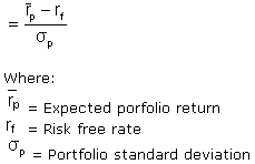
The Sharpe Ratio is a well-known measure of portfolio performance. It is a ratio that allows for the comparison of various portfolios and allows for the measurement of their profitability. The mathematical definition is described as a division between the expected rate of return subtracted by the risk-free rate of return and the standard deviation of rates of return [6].

In practice, the ratio is calculated annually:

The ratio describes how much excess return you are receiving for the extra volatility that you endure for holding a riskier asset ([1]). In simple words, the higher Sharpe Ratio is, the more portfolio is profitable.

Why is the Sharpe ratio so popular?

Most traders are still using the Sharpe Ratio because of its simplicity and ease of interpretation. It was proposed by Sharpe in 1966 and became credible to most users due to Nobel Prize in Economics for his works on the Capital Asset Pricing Model ([5]).

Properties of the Sharpe Ratio

With reference to [1], the ratio has several properties. It is immune to manipulation by leverage. It can be interpreted as a T-statistics to test the hypothesis (see [8]) that the return on the portfolio is equal to the risk-free rate of return. The higher ratio is consistent with a higher probability that the portfolio return will exceed the risk-free return. The investor using the ratio has a utility (see [7]) whose only arguments are expectation and variance of returns.

Forgotten assumptions

Unfortunately, most traders forget that the Sharpe Ratio doesn’t apply to every data set. The central assumption of the ratio is that the distribution of the returns is normal. The financial market should be frictionless (without financial costs), and the risk-free rate of return should be constant and identical for lending and borrowing. Also, data used for computation should contain the initial capital of the portfolio.

Consequences of the ratio

Even though it is really hard to obtain the normality of returns on every possible data, the Sharpe Ratio has other disadvantages, which are represented in [1].

The ratio does not quantify the value added, and it’s only a ranking criterion. It has a hard interpretation when the value is negative. The Sharpe ratio does not make any distinction between upside risk and downside risk.

In the case of aggregation of portfolios, the correlation between volatilities is not included in the ratio. It is suitable for investors who invest in only one fund.

It doesn’t refer to a benchmark. The choice of a risk-free rate is rather important, though the impact is weak. The result highly depends on the initial capital of the portfolio.

The sampling error of standard deviation is embedded in the values of the ratio. By using the standard deviation of returns, the Sharpe measure puts both positive and negative variations from the average on the same level. But most investors are only afraid of negative variations.

As a consequence, the Sharpe Ratio leads to inappropriate results on particular sets of data.

When the ratio fails

To be aware of how important the assumptions are, consider the following example [*]:

When the expected return is negative, the Sharpe Ratio gives the inappropriate answer. The Sharpe Ratio from Instrument A should be greater than that from Instrument B.

INVESTMENT A				SHARPE RATIO
TOTAL RETURN	-10.00%			-1.5
RISK-FREE RATE	5.00%	NUMERATOR	-15.00%
STANDARD DEVIATION	10.00%	DENOMINATOR	10.00%

INVESTMENT B				SHARPE RATIO
TOTAL RETURN	-10.00%			-0.92
RISK-FREE RATE	5.00%	NUMERATOR	-15.00%
STANDARD DEVIATION	16.25%	DENOMINATOR	16.25%

The solution to Negative Returns

In the case of negative returns, the Israelsen modification of a Sharpe Ratio gives appropriate results. This ratio could be used as a verifying measure of a standard Sharpe Ratio (the values are meaningless, but the order remains accurate).

The Israelsen modification of the Sharpe Ratio from a previous example provides that Instrument A is greater than the Sharpe Ratio from Instrument B.

INVESTMENT A				SHARPE RATIO ISRAELSEN
TOTAL RETURN	-10.00%			-0.015
RISK-FREE RATE	5.00%	NUMERATOR	-15.00%
STANDARD DEVIATION	10.00%	DENOMINATOR	10.00%

INVESTMENT B				SHARPE RATIO ISRAELSEN
TOTAL RETURN	-10.00%			-0.024
RISK-FREE RATE	5.00%	NUMERATOR	-15.00%
STANDARD DEVIATION	16.25%	DENOMINATOR	16.25%

In conclusion, when negative returns occur, the investor should also check the value of the Israelsen modification before making the decision.

Avoiding invalid distribution

The most dangerous ratio usage is when the distribution of the returns isn’t normal. It seems that the best idea is to check the normality of the returns before use of the Sharpe Ratio. Several statistical tests can validate data distribution, such as Shapiro Wilk, Anderson Darling, Cramer von Misses, Dagostino Pearson, Jarque Berra, Kolmogorov Smirnov, Kolmogorov Lilliefors, Shapiro Francia (see [9]).

Generalizing Sharpe Ratio

On the other hand, there are different extensions of the Sharpe Ratio, which gives more accurate results by extending different assumptions. There are plenty of them described in [1], but only those with skewness and kurtosis will be presented.

Skewness describes the asymmetry of the probability distribution. If there are more extreme returns extending to the right tail of a distribution, it is said to be positively skewed, and if they are more returns extending to the left, it is said to be negatively skewed [2].

Kurtosis provides additional information about the shape of a return distribution. Formally it measures the weight of returns in the tails of the distribution relative to standard deviation but is more often associated with a measure of flatness or peakedness of the return distribution [2].

Skewness and Kurtosis are normalized forms of 3rd and 4th central moments, respectively (see [10]). Its combination with the Sharpe Ratio allows for approximating the ratio when the distribution is not normal. This method leads to the proposition from [4], where skewness divided by kurtosis is added to the Sharpe Ratio, which results in a new performance measure.

In the case when the owner of the portfolio has different preferences (different utility – see [7]), there are other ratios to measure the performance. The Adjusted for Skewness Sharpe Ratio allows measuring the performance using hyperbolic absolute risk aversion (HARA), constant relative risk aversion (CARA), or constant absolute risk aversion (CRRA). More details can be found in [3].

Conclusion

The Sharpe Ratio is a standard measure of portfolio performance. Due to its simplicity and ease of interpretation, it is one of the most popular indexes. Unfortunately, most users forget the assumptions and that results in an inappropriate outcome. They should consider checking the distribution of the returns or validating the results with other performance measures before making a decision on the market.